Excel Course - Beginner to Advanced - Udemy Notes - Basic operations in Excel and how to do it

 

Ribbon tab - the top tool-bar of the Excel Sheets 

Formula bar - the bar below the Ribbon Tab of the excel sheet

Status bar - the bottom most tool bar where you can zoom in and zoom out of an excel sheet

Excel workbook - A sheet of an excel, where it is made up of Rows and columns - it has about some 1,048,576 ROWS and 16,384 COLUMNS 

Upto 256 Sheets can be added for Excel to optimally work, but then the limit on the number of sheets that can be added totally depends on the Processing power of the CPU

To change the number type format

·         Home -> number format -> change the type of number format

Relative reference

It refers to the way by which Cells across another locations can be referenced and used from some other cell position - Example as given below, Values from B4 to B8 can be referenced and added in another totally different position

ABSOLUTE REFERENCE - When some cells are referenced by absolute reference then the reference of it does not change when the formulas are extended across Other cells

To use absolute reference use a dollar sign before it

For eg – E5/$E$9

• ·     Totally there are 461 functions built in Ms Excel

Dragging around the data In excel

In same worksheet

Select all the data and move them around by left clicking and holding at around the corner of the selection, like shown in the figure below

Different worksheet

Just copy/cut and paste it in the required location 

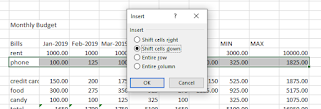
Adding new Row and columns

Select the entire row by holding cntr + shift

After selecting the rows hold control and '+' on the num pad , a dialogue box will open as shown below and now choose entire row option 

Similarly do for Column also.

Like shown in the above figure , this is also an another way to insert columns

Deleting Rows and Columns

Similar to inserting select either the row/column and then click "control + '-' " 

Changing the size of rows and columns

Select the row or Columns and double click at the place as shown in the below figure

Similarly you can do so for all the data by selecting all the rows and columns and double clicking at any of the exact place between the borders of the cells

If you do these then the rows and columns would be automatically adjusted to the size of the biggest entity in that particular row/column.

In case if the cell is small, the corresponding Numeric value inside would be displayed as set of hashes, in case of texts it would be cut out the display

Hiding the Rows and Columns

Like shown in the above figure, select a row/column and right click on it to display a little menu, inside that choose 'Hide' option in order to hide the row/column.

Likewise you can hide/unhide multiple rows and columns, using similar such method

Inserting/Deleting/Renaming Worksheets

Right click on the Sheet 1 button, Below the window and select the command you want to execute 

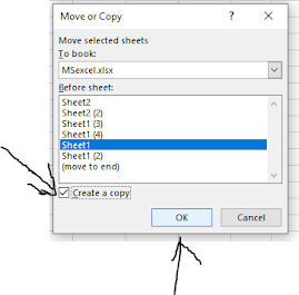
Move or Copy new sheets

Pressing control left click on the sheet1(4) tab and drag it to the next bar, and drop it,then you can see that a new sheet has been created 

Another method is by right clicking on the sheet tab and choosing move or copy option then selecting the position as shown above and clicking OK

Adding borders

Method - 1 

select Home button , under that tool bar select the little square box after B I U tab, and choose whichever border you want.

Method -  2

Under Home toolbar, select format bar inside that choose format cells

Inside the format cells, customise the border that you want for the choosen block of cells, as shown below -

Formatting the values of a Column/Row

Under the home tool bar , Goto general and change the format of the column/row of values into Number,Currency, Long date, Short date, Accounting etc 

Format painter 

if you like the look of a particular block of excel and want to imitate that to other block of excel then do this , 

choose the block of cells whose look you want to copy then goto home and choose on format painter option as shown below, and apply it on the target BLOCK.

Clear all the formats of a cell 

Goto home bar and click on clear and select clear formats to remove all the formats of a particular cell

Creating a new format style

First select the cell whose format you want to save, then from the home tab, select the cell styles , and click into new cell style

and the name the new style and click on 'OK'. Thus, now the cell style is saved and whenever you want to use it, click on cell styles and just apply it

You can also modify the fill color and everything by selecting the format button and changing inside it. 

Merge and center the Cells

To merge some particular cells and center the content inside it, select the particular bunch of cells that needs to be merged and click on Merge & Center from Home tool bar and select it.

Perform Conditional Formatting

On the home tool bar , select conditional formatting as shown above and apply the conditions from the given list of sub-options

Inserting pictures , shapes , Smartarts

Pictures, smart arts and shapes can be inserted from the toolbar as shown above and these shapes can even be formatted with and played around